
Simplifying technology and system component models in RA can lead to under or over estimating system risk, leading to incorrect adequacy assessments. On the other hand, overly complex models may be too computationally expensive. Selecting appropriate modeling options can help avoid these pitfalls and increase the accuracy of adequacy assessments. This page provides information regarding the breadth of options available to model conventional and emerging technologies and system components in resource adequacy.
Information regarding the modeling of the following technologies and system components are addressed in this site:

A tabulated summary of modeling approaches by level of fidelity is provided for each technology and system component to provide a summarized set of modeling options for practitioners. Three levels of modeling fidelity are proposed, outlined below.
LEVEL I
Most basic models: may be sufficient when system reliance on technology addressed is low.
LEVEL II
Mid-fidelity models: may employ advanced modeling techniques for certain aspects of a technology and basic ones for others.
LEVEL III
Highest fidelity models: these models systematically capture technology behavior with the highest level of accuracy compared to Levels I and II and generally employ state-of-the-art modeling approaches.
THERMAL GENERATION
Background
Thermal generation resources are grouped in three main thermodynamic cycle classes: Rankine cycle, Brayton cycle and reciprocating internal combustion engine (RICE). While other classifications schemes (e.g., fuel source) could be considered, plant availability is most impacted by the design of the resource.
Cycle | Description | Flexibility | Fuels |
|---|---|---|---|
Rankine | Steam turbine and boiler or heat recovery steam generator (HRSG) | Lower | Uranium, Coal, Fuel oil, Gas, Waste, Biomass, Peat, Geothermal, Hydrogen |
Brayton | Combustion turbine | Higher | Gas, Distillate, Synthetic gas, Hydrogen, Ammonia |
RICE | Engines | Higher | Diesel, Distillate |
There are two notable resource types that combine elements of two cycles: combined cycle gas turbines (CCGT) and combined heat and power (CHP). The case of CCGT incorporates some combination of combustion turbines and steam turbines with intermediate heat recovery in a variety of potential configurations. In the case of CHP, combustion leads to the raising of steam within boilers. Steam is then used to both generate electricity in a steam turbine and then either provide process steam or feed heating water circuits.
All thermal plants can respond to dispatch instructions, though response rates vary based on both plant design, the availability of fuel, and operational conditions. RICE and aeroderivative gas turbines respond the fastest and may sustain flexible operation over extended periods, at the expense of part load efficiency penalties. Rankine cycle steam units can also respond, but over a longer time frame, that is limited by thermal properties of the plant components, boiler dynamics, the operation of coal mills, and management of reactor cores. New forms of thermal resources, such as small modular reactors or hydrogen turbines, are under active development but fit within the framework presented. The availability, efficiency, and flexibility of each of these plant and fuel types is dependent on a number of factors as summarized in the table below.
Cycle | Factors influencing availability | Factors influencing efficiency | ||
Common factors | Specific factors | Common factors | Specific factors | |
Rankine | Fuel, | Secondary fuel capability & storage |
| Coolant source / sink temperature |
Brayton | Fuel supply logistics | External air temperature | ||
RICE | External air temperature | |||
Modeling Options
Capacity available for dispatch is understood as the maximum output that a resource can sustain for an extended period, excluding the impact of:
- Maintenance
- Fuel supply interruption
- Forced outage related causes
LEVEL I:
Maximum generating or contractually declared capacity.
Declared capacity for dispatch commonly represents the plant's self-assessment of the capacity available for dispatch at a given time. It is generally known with high certainty hours to days ahead when weather and fuel availability is well established. Further out, it may be estimated based on contractual obligations to provide capacity in capacity markets.
Maximum generating capacity may be reduced when any factor influencing efficiency becomes active, such as high temperature derating.
LEVEL II:
Seasonally adjusted capacity rating on top of Level I approaches or declared capacity for dispatch for short-term assessments.
Seasonally adjusted ratings are derived based on climatological assessments of the temperature at the plant location and assessed on a plant-by-plant basis, reflecting the design, location, and other plant specific factors.
LEVEL III:
Condition-based capacity rating, incorporating a range of forecasted conditions such as temperature, emissions limits, or availability of cooling water to estimate the maximum production capacity of a plant under a given condition at a specific time. When these conditions are triggered in a model, an update to the expected capacity available for dispatch can be made. This approach is typically not implemented in long-term resource adequacy studies but may be in short-term studies given the extensive data input required.
Asset Availability: Maintenance and Forced Outages
Resource availability represents a given unit’s capability to deliver its declared capacity available for dispatch at any time, considering the possibility of maintenance or forced outages occurring. Maintenance and forced outage factors are typically considered separately, given the ability to schedule maintenance at a specific time or potentially recall the resource faster than anticipated.
Maintenance Outages
Approaches to incorporate maintenance outages in RA depend on the scope of the study. In the season- to days-ahead time frame, maintenance schedule information, indicating maintenance timing and duration, is likely to be available for most resources. The availability of this information greatly reduces the uncertainty associated with estimating the set of available units during a study period. Considerable uncertainty arises in the timing and nature of planned resource maintenance periods that are years or decades ahead. While maintenance is highly likely to continue to be scheduled during the periods of lowest system stress, as illustrated below, the timing of such periods may be less certain and have varying durations.

Research into, and experience with, the operation and reliability of thermal plants also points to the changing nature of operation and maintenance (O&M) activities as plants change operational mode to provide more flexibility across fewer running hours. The impact of flexible operations varies depending on plant type, location, the extent of cycling, hot and cold starts carried out, as well as individual plant strategies. While, at present, major work is typically focused on one or two extended maintenance periods per year requiring a plant outage, as illustrated in the figure to the left, future O&M strategies are likely to adapt to the extent they can, to shorter and less certain maintenance windows.
LEVEL I:
Heuristic maintenance schedules are employed to schedule resources for maintenance based on past operational data. A valley filling approach may be employed, scheduling maintenance events based on the size and duration of the resource outage in descending order and aligned with minimizing the forecasted net load profile. Most dedicated RA tools implement a version of this to generate a reasonable approximation to maintenance schedules.
LEVEL II:
Optimized maintenance schedules for long-term assessments and forecasted maintenance schedules for short or near-term assessments.
Optimized maintenance schedules apply a pre-processing optimization to schedule the set of maintenance events across a study period using forecasted demand and renewables profiles as well as maintenance profiles by asset type. Optimization functions are typically formulated to reduce the potential for system stress, similar to the heuristic method. Delay and recall may be modeled by including the option to curtail maintenance and by generating additional maintenance samples testing the impact of unexpectedly prolonged maintenance periods.
Forecasted maintenance schedules are known in advance and updated based on progress. This information is provided as an input into the RA assessment directly. For assets with no declared maintenance but where maintenance is likely, the heuristic approach can be taken to fill in expected maintenance based on forecasted conditions. Forecasted maintenance schedules are common practice for short term assessments.
LEVEL III:
Optimized (long-term) or forecasted (short or near- term) maintenance schedules with provisions for delays and recall are used for maintenance modeling.
Provisions for delays and recalls account for the ability to recall a limited amount of ongoing maintenance under emergency conditions, informed by operational experience and the nature of the assets under maintenance.
There are two categories of approaches to model forced outages: deterministic and probabilistic. The general characteristics of each approach differ substantially, meaning that either may be more or less suited to different use cases:
- Deterministic methods entail the estimation of the likely availability of a resource type over an assessment period and aggregate resource availability to develop a supply-side availability profile. Examples include:
- Performance during the top ten demand periods across a three-year sliding window
- Historical performance during conditions defined by capacity market rules
- Probabilistic approaches aim to represent the stochastic nature of the failure and repair of generating resources, reflecting the variance in resource availability that is possible at any moment. Probabilistic methods fall into two general approaches: analytical and simulation Both approaches rely on the same standard variables – a failure rate, a repair rate, and their derivatives. These rates govern the transition of a resource between availability states in a Markov process. The most common configuration of states is a two-state model (available and unavailable) that is stationary over time.
In analytical approaches, the probability that a unit is in the available and unavailable state at any point in time is derived from its failure and repair rates. The most used derivative variable is the Equivalent Forced Outage Rate (EFOR) or the Equivalent Forced Outage Rate on Demand (EFORd), representing the probability that a unit is unavailable, in the latter case conditional on periods when the resource would be required to meet demand.
The analytical approach has some implicit assumptions, inherent to many adequacy studies and that modelers need to be aware of:
- Each resource’s behavior is assumed independent of others.
- Failure and repair rates are typically assumed to be stationary.
- Resource availability in one interval is independent from the previous interval.
- It is assumed that operational, or energy-related, constraints do not limit the availability of a resource.
Simulation based approaches typically rely on Markov Chain Monte Carlo (MCMC) simulations. Here, the evolution of generator availability from one interval to the next is modeled by drawing a random variable, and then evaluating whether its value corresponds to a change in state at a given time – either moving to an unavailable state from available or from unavailable to available. Since this approach draws a random variable in each interval, multiple samples need to be studied to achieve convergence of the ultimate risk metric (LOLE, EUE, or other). The addition of further states, such as available and offline and available and online, allows for start-up failure to be modelled. This feature may become increasingly important in systems with significant ramping requirements, when multiple units start in close succession to meet a net load ramp, potentially during adverse conditions.
For each sample, there is a definitive MW capacity available or unavailable in each interval, as compared to the analytic approach where a probability of exceedance is used for given capacity levels. This approach therefore allows for other considerations in system
LEVEL I:
Monte Carlo Markov Chain (MCMC) hourly simulation with seasonally adjusted forced outage rates.
- A Monte Carlo sampling approach is applied to generate hourly profiles of generator availability using at least a two-state Markov Chain model, modeling available and unavailable states.
- The failure and repair rate used should change on a seasonal basis to be commensurate with the projected seasonal average Effective Forced Outage Rate.
This methodology is available across many commercial and research adequacy assessment tools. The benefits of the MCMC simulation approach when compared to the convolution approach is that individual asset availability can be queried at any hour, allowing for system level optimization or simulation to consider the loss of a specific asset, rather than the expected cumulative unavailability of the resource fleet taken in aggregate. Simulation-based approaches also preserve inter-temporal state transitions, an important feature that enables the consideration of energy and flexibility constraints as part of overall system modeling.
LEVEL II:
Monte Carlo Markov Chain hourly (MCMC) simulation model with daily condition-based failure rates.
An advance upon seasonal rates (explained in level I) is to consider condition-based failure rates that are updated on a daily basis. In such a case, the failure and repair rates are determined for each unit for each day based on a trigger condition associated with that day, such as mean temperature or wildfire risk. No other changes are required to the MCMC simulation approach. Daily failure rates are recommended in any system where thermal resources are exposed to temperatures below 32°F (0°C) or above 95°F (35°C).
LEVEL III:
Monte Carlo Markov Chain (MCMC) hourly simulation model incorporating weather dependent/condition-based failure rates by interval.
Level III models improve further by updating failure rates based on the conditions present in each simulation interval, allowing for improved granularity about the timing of return to service and failure within a day as conditions deteriorate. Implementation of this approach does not influence the core MCMC process but does require updates to the failure and repair simulation parameters that may require changes to certain adequacy assessment tool capabilities.
Aside from failure while running online and constraints in changing dispatch setpoint, generators can fail to transition between offline and online. Start-up failure is an issue of importance due to the potential for generators to fail at the same time as net demand is increasing. Failure to start is often different from forced outage failure in that, in many cases, the failure is related to start procedure issues and may be quickly recovered. With greater projected net load variability, cycling of generating assets is likely to increase. With increased cycling, a greater potential opportunity arises for startup failure.
Start failure can only be modelled in simulation approaches where generator dispatches are included. Such methods are typically combined with MCMC forced outage modeling. The standard practice in RA has been to not include start up failure on the grounds that thermal generation do not experience frequent cycling.
LEVEL I:
Failure to start is not included in RA model.
LEVEL II:
Under cases where thermal generation is exposed to increased cycling, beyond its original intended operating profile, or has passed the midpoint in the asset's design age, including a model for start-up failure becomes recommended practice. Start-up failure models can be implemented using a Markov Chain process that is contingent on the generator being started by a chronological dispatch model. When a generator is committed after being offline a post-processing step overlays the failure state. This may, or may not, result in load shedding depending on the system state.
LEVEL III:
Condition based start failure is modelled for failure to start.
In systems where thermal resources are exposed and vulnerable to common cause start failure, such as cold weather in regions with low hardening to such conditions, startup failure rates estimates may be varied based on the prevailing condition (e.g., temperature). The application of this method is restricted based on the data available similar to conditional forced outage assessment.
Limitations associated with fuel supply may also need to be considered for thermal resources. While energy constraints have traditionally been associated with hydro and energy storage resources, increasing emphasis has been placed on the energy constraints associated with gas, liquid fuel, and dual fuel resources.
Constrained gas supply and reliance on liquified natural gas (LNG) or gas storage for units with limited on-site fuel storage have become more commonplace. Coal units may have sufficient fuel on site but during cold conditions, frozen coal piles or non-performant fuel handling equipment may result in reduced fuel availability to a plant.
The table below outlines common fuel delivery risks by fuel source.
|
Fuel source |
Risk Influencing Factor |
Trigger Condition |
|
Natural Gas |
Pipeline supply restrictions due to local gas demand priority |
Cold weather |
|
Pipeline supply restrictions due to gas infrastructure outages |
Multiple, including cold weather |
|
|
Insufficient LNG inventory |
LNG prices, LNG infrastructure availability |
|
|
Uranium |
Prolonged refueling outages |
Plant or fuel condition |
|
Reduced operational range based for crud management |
Fuel cycle |
|
|
Coal |
Coal pile freeze |
Cold weather |
|
Coal supply constraint, waterway |
Drought |
|
|
Coal supply constraint, rail |
Floods, rail infrastructure damage |
|
|
Oil |
Insufficient inventory resupply |
Cold weather, flooding |
|
Distillate |
Insufficient inventory resupply |
Cold weather, flooding |
|
Biomass |
Unavailability of fuel source |
Drought, flood, travel constraint |
|
Varying calorific value of feedstock |
|
|
|
Hydrogen |
H2 inventory |
Renewable production, or other |
Similarly, emissions constraints may limit the running hours of resources, potentially reducing plant availability during unforeseen periods of system stress. In many cases these emissions limits may be lifted under emergency situations, but in an ideal case these would be planned against at the outset.
EPRI developed the Resource Adequacy Fuel Insufficiency Screening (RAFIS) tool to support planners in examining potential system gas limits and impacts on adequacy as a support tool for adequacy assessments.
LEVEL I:
No model of energy limits is considered.
This is the standard modeling approach for thermal resources in many adequacy studies today, operating under the assumption that thermal resource operators will have sufficient foresight or back-up options to procure and manage fuel in order to meet any potential system stress conditions. It is also envisaged that emissions limits would be removed when a system faces a high likelihood of load shedding, making those limitations immaterial to reliability outcomes.
LEVEL II:
A fuel pool is modeled for energy limits.
Fuel pool models are suitable within chronological MCMC RA simulations. A constraint is introduced to limit fuel consumption for a set of generators reflecting the assumed availability of that fuel. Simplified heat rate and start up heat estimates are made for each resource associated with a fuel group to produce an estimate of the fuel demand required by the resource set. This is then limited by a daily or weekly fuel availability, representing the gas pipeline and LNG daily contracted or delivery capacity, net of non-power demand for gas (e.g., residential gas consumption).
Fuel pool constraints are recommended if gas supply is known to be a limiting factor in operations, additional gas supply is required to facilitate the addition of new generating capacity, significant additional gas demand is forecasted downstream of the study region, or in cases where rapid population growth is forecasted to increase the demand for natural gas in a region. For dual fuel units it is recommended that resources be associated with the central fuel pool for the primary fuel source and to include secondary constraint on the availability of the secondary fuel in line with site storage capability and realizable fuel deliveries by day. A similar approach can be taken to associate resources with two fuel pools, representing firm and non-firm fuel supply pools in cases where generators are known to depend significantly on spot gas contracts.
LEVEL III:
Hourly fuel offtake limits and fuel pool are modeled.
In cases where daily pipeline capacity does not offer an accurate representation of the gas available to generators, time of day related constraints affect the availability gas supply to power plants, or downstream fuel supply is prone to weather related outages, it is recommended to model energy limits at an hourly granularity and, where data permits, to incorporate condition-based fuel supply estimates. Derating of fuel supply based on temperature, environmental or other condition should be based on a data supported approach. These constraints have the same form as the fuel pool but with a smaller time constant.
Flexibility constraints are the most recent modeling consideration to be added to resource adequacy assessments. In the past, flexibility issues, where they did arise, were mostly related to the change in setpoint around an hour-long interval, resulting in frequency excursions. As such, resource adequacy assessment was initially developed around the principal that flexibility issues, such as they existed, were operational timeframe constraints that could be resolved by means available to dispatchers. The need for flexibility was not so great that it would present the basis on which resource investment would be required to mitigate.
As grids incorporate greater shares of wind and solar power, the operational uncertainty and variability that systems face can be considerably greater than in the past and may exceed the magnitude of what can be managed exclusively through operational means. Previous assessments have shown the potential for flexibility constraints to have a material impact upon the estimation of LOLE.1 Forward monitoring and assessment of the potential for load shedding to be driven by flexibility related limitations may be critical, particularly while grids are transitioning from legacy to future-state generation mixes. These assessments require chronological simulation and the addition of some operational policies, such as operating reserve and advanced storage modeling. The need to model RA at a sub-hourly resolution may also need to be considered in flexibility-constrained systems, however computational limitations may need to be addressed. EPRI has previously investigated methods for assessing system flexibility needs including a discussion of when sub-hourly modeling may be beneficial for ensuring sufficient operational flexibility.2
In practice, most analyses do not include flexibility constraints associated with thermal generation. This is likely to remain valid for systems that do not experience net load ramping substantially exceeding historical demand ramps and sustains a hydro-thermal fleet where a significant portion of the resources are able to start and stop within the same day on a consistent basis.
Read More:
LEVEL I:
No modeling of flexibility constraints.
This is likely to remain valid for systems that do not experience net load ramping substantially exceeding historical demand ramps and sustain a hydro-thermal fleet where a significant portion of the resources are able to start and stop within the same day on a consistent basis.
LEVEL II:
Minimum generation, minimum up/ down time constraints.
For most systems, the first instance in which the addition of flexibility is recommended occurs when the forecasted net load profile displays a midday valley (e.g., a duck curve), with a delta in peak to valley net load approximately equivalent to the addition of fast start thermal, battery storage, and demand response resources available to the system. Under this scenario, the potential exists for traditionally inflexibly operated plants to be required to cycle, particularly during maintenance periods for peaking plant. It is recommended that the addition of minimum online generation and minimum up and down time constraints be added to the simulation model in order to capture issues related to minimum turn down, and double-two-shift cycling of thermal plant. The addition of those constraints represents a minimum required to diagnose the potential for flexibility shortfalls owing to commitment-related limitations. Commitment-related constraints are known to considerably increase the time associated with the execution of simulations, limiting RA analyses to a reduced number of samples. Adaptive approaches to screening net load profiles for potential flexibility related constraints are under exploration but may aid support in sample scenario selection in future.
LEVEL III:
Advanced constraints plus start-up and ramp rates are modeled.
In cases where the magnitude of the midday valley to peak range exceeds the capacity of fast responding resources and demand response, the addition of startup time and ramp rate constraints, on top of Level II constraints, to the operational simulation may be warranted. The addition of such constraints significantly increases run time and may only be required as a supplementary check after an initial screening process.
Open Modeling Gaps
Thermal modeling approaches have evolved over the past 70 years in response to changing technologies, exposure to risk, and common cause events. Thermal resources will likely continue to play an important role in many low carbon systems, so understanding how to accurately represent them in RA in the context of evolving power systems is essential. A set of open modeling gaps relating to thermal power generation is presented in the Table below.
Table: Open modeling gaps relevant across technology models, data collection, and tools.
|
Modeling Approach |
Gap |
Severity |
Comment |
|
Capacity Limits |
Cooling water |
Low |
Derating owing to reduced cooling water availability or elevated temperatures in ultimate heat sinks is a challenge to implement (models) and estimate (data) from a long-term planning point of view. Targeted scenario analysis or stress testing may be a prudent approach under such circumstances. |
|
Asset Availabiltiy |
Time and condition-based outage rates |
High |
The integration of condition and time-dependent failures and repair rates requires improved estimates (data), modeling approaches (models) and integration into tools (tools). Studies that implement condition-based outage rates can be achieved at present, but largely through extensive scripting and with limited consistency between approaches. |
|
Maintenance forecasting |
Medium |
As net loads evolve, traditional shoulder maintenance seasons may be at elevated risk of load shedding should maintenance practices remain unchanged. Anticipating how maintenance strategies will evolve (data) and how to approximate that behavior in adequacy assessments (models) will play a significant role in determining risk during the shoulder months. |
|
|
Maintenance recall |
Low |
The ability to recall resources from ongoing maintenance is an operational time frame action that can be taken to reduce the impact or likelihood of load shedding. Building an estimate (data) and approach to recall a portion of plant on maintenance during load shedding events is likely to be material to the outcome of adequacy studies (models). |
|
|
Energy Limitations |
Fuel networks |
Medium |
In cases where the performance of fuel delivery networks requires more granular representation than that achieved through a fuel pool or hourly offtake constraint implementation, fuel network elements (e.g., compressors, pipelines, extraction facilities) may need improved representation within adequacy studies. This is currently an open gap to determine the level of detail and functionality that would be required in such as case. |
|
Emissions limits |
Low |
Medium term scheduling may be required in cases where emissions limits require reduction in available capacity and when stressful conditions may be anticipated with high certainty. |
|
|
Flexibiltiy Limitations |
Impact of carbon capture |
Low |
The potential addition or retrofit of carbon capture technology at thermal power plants may alter the flexibility profile of the resources resulting in a need to assess flexibility in a wider range of conditions than carried out at present. |
VARIABLE RENEWABLE ENERGY
Background
Although onshore wind, offshore wind, solar PV, and concentrating solar power are all different technologies, they are modeled similarly within resource adequacy studies and therefore addressed together here. Because of the dependence of variable renewable energy (VRE) on stochastic weather phenomena, representing VRE generation is an important source of uncertainty to capture in RA modeling. Unlike technologies like coal, natural gas, and nuclear generation, the output of VRE is strictly dependent on environmental factors: mainly wind speed and solar irradiance. Historically, VRE outputs have been treated as non-dispatchable resources: they could be curtailed but did not generally participate in real-time electricity markets. However, with the development of advanced control strategies, VRE units can provide a range of grid services, including frequency regulation and synthetic inertia, much like conventional generators, within the envelope allowed by varying environmental conditions.
Modeling Options
Certain RA studies still model VRE using a fixed capacity derate, which may be calculated based on median net real power output during pre-determined reliability hours. While significantly simplifying modeling, this approach doesn’t account for the impact that hour-to-hour wind variability can have on the system. The use of pre-determined reliability hours also presupposes a perfect foresight of at-risk adequacy periods which may not hold true in all scenarios, especially as increased renewable and storage buildouts are shifting periods of peak risk. As such, it is a widely accepted best practice, and recommended here, for VRE generation to be modeled using timeseries.
Timeseries data can be either collected from historical plant operating data, or by using remotely sensed or reanalysis data generated from weather records. Synthetic data is often utilized in cases where there has not been any VRE capacity installed at a specific geographical location. For all technology types, a large number of weather years are required to fully capture weather-driven uncertainty and extreme weather events. The specific number of years depends on the region and the relative share of VRE. It is recommended that this should be examined for each system by looking at longer datasets before determining whether shorter sets could be used. Additionally, care should be taken to ensure correlated weather year data is used across all weather-dependent technology and load models – this includes wind and solar data, but also load data and any temperature dependent data – such as temperature-dependent outages or demand response. Further information on best practices for timeseries creation can be found in Data Guidelines.
Aggregation of wind and solar plants within resource adequacy models is often used to reduce model complexity and overcome data availability issues. Aggregation involves summing hourly generation over a geographical region, often across a climatic zone, to produce an equivalent aggregated generation profile. These aggregated units are then included in the overall resource adequacy model as if they are a single unit.
Resource Availability - There are a number of factors that can impact the ability of wind and solar plants to generate electricity. These include planned and forced outages due to equipment maintenance or malfunction, but also unavailability or reduction in generation due to environmental factors, such as pollen accumulation or snow cover for solar PV plants, or blade icing for wind turbines. Additionally, age-related degradation can impact power delivery over the unit’s lifetime.
It is general practice in most resource adequacy models to date to implicitly incorporate these factors affecting resource availability within the power generation timeseries, rather than explicitly modeling them. This is because historical generation data is usually reported inclusive of outages and derates. Furthermore, outage data for solar and wind installations is often unavailable or of poor quality. Finally, including these derates and outages implicitly as part of the generation timeseries decreases the resource adequacy model complexity. Future efforts may be required to more explicitly model outages, for example during cold weather or dust storms, where outages might be higher than a weather timeseries alone may suggest.
LEVEL I:
Fixed capacity derate calculated based on estimated power output during stress periods.
While significantly simplifying modeling, this approach doesn’t account for the impact that hour-to-hour wind variability can have on the system. The use of pre-determined reliability hours also presupposes a perfect foresight of at-risk adequacy periods which may not hold true in all scenarios, especially as increased renewable and storage buildouts are shifting periods of peak risk.
LEVEL II:
Several years to decades of hourly data and correlation amongst weather-dependent generation, outages, and load shapes.
It is a widely accepted best practice, and recommended here, for VRE generation to be modeled using timeseries.
Timeseries data can be either collected from historical plant operating data, or by using remotely sensed or reanalysis data generated from weather records. For offshore wind power plants, or all types of VRE in regions with less current installed capacities, synthetic data is often utilized due to the limited availability of historical data. For all technology types, a large number of weather years are required to fully capture weather-driven uncertainty and extreme weather events. The specific number of years depends on the region and the relative share of VRE. It is recommended that this should be examined for the system by looking at longer datasets to determine whether shorter sets could be used. Additionally, care should be taken to ensure correlated weather year data is used across all weather-dependent technology and load models – this includes wind and solar data, but also load data and any temperature dependent data – such as temperature-dependent outages or demand response. Further information on best practices for timeseries creation can be found in the Data Collection Guidelines page.
LEVEL III:
Several decades of hourly data, with correlation amongst weather shapes enforced and consideration of operational forecast uncertainty.
The difference between level II and III is that level III looks at a longer time period of data (several decades) and operational forecast uncertainty is included.
Historically, VRE operational forecast uncertainty was not considered in resource adequacy modeling. Today, certain tools are starting to include operational constraints, to evaluate whether the system has sufficiently flexible capacity to respond to potential shortfall events. Accounting for operational forecast uncertainty may be material to RA outcomes for systems with sufficiently high levels of VRE shares and is recommended to be examined in regions where shares are above 25%-30% annual energy penetration, if not lower.
Open Modelling Gaps
Resource adequacy models for variable renewable energy are relatively well established and in widespread use. Two primary gaps remain that need to be addressed as VRE shares continue to grow. First, the collection of appropriate and good quality data informing weather- dependent, correlated, VRE power outputs and outages. Secondly, further understanding the need, and establishing industry standards, for modeling VRE output uncertainty within RA.
STORAGE AND HYBRID POWER PLANTS
Background
The focus of this section is on bulk storage and hybrid power plants. The most prevalent for grid-scale applications are pumped storage hydro (PSH) and batteries. Other, less prevalent, types of storage include flywheels, compressed air energy storage (CAES), and molten salt (thermal) storage.1 This section focuses primarily on short-term storage, which is mostly cycled daily, sometimes across several days. Most considerations specific to long-term storage are addressed in the Hydropower Section.
Read More:
Modeling Options
The most common approaches to model energy storage (ES) dispatch in RA assessments are:
- Approximating storage operations by modeling it as a thermal unit
- Using heuristic dispatch models (often within heuristic tools)
- Modeling storage operations through timeseries based on historical data
- Explicit modeling of storage dispatch and state of charge within 8760 optimizations
Read more:
LEVEL I:
- Option 1: Storage operations are not explicitly modeled; they are implicitly accounted for in net-load profiles.
- Option 2: Storage is modeled as a marginal thermal unit, assuming capacity is available during shortfall events.
- Option 3: Storage is dispatched based on generation shortfall prevention heuristics: ES discharges only when the system is at risk of a loss of load event.
The most basic ES dispatch modeling involves modeling ES as a thermal unit (option 2), assuming full availability during times of system stress, or exogenously including expected ES operations through timeseries based on historical operational data that may be netted from system demand. The thermal unit approximation method can assume that storage is only dispatched during high system stress time periods at a high marginal cost, mostly limiting its usage to providing RA support. The thermal unit approximation also assumes that storage is fully charged prior to risk hours. Neither the thermal unit approximation nor the timeseries methods explicitly models storage intertemporal constraints, reducing the complexity of RA model formulations. However, modeling ES
LEVEL II:
Storage economic dispatch is modeled through in 8760 optimizations, explicitly modeling linked storage dispatch and state of charge.
This is the recommended approach for any regions where storage is non-negligible (e.g., installed capacity is more than 1%-2% of peak demand).
LEVEL III:
Several decades of hourly data, with correlation amongst weather shapes enforced and consideration of operational forecast uncertainty.
The difference between level II and III is that level III looks at a longer time period of data (several decades) and operational forecast uncertainty is included.
Historically, VRE operational forecast uncertainty was not considered in resource adequacy modeling. Today, certain tools are starting to include operational constraints, to evaluate whether the system has sufficiently flexible capacity to respond to potential shortfall events. Accounting for operational forecast uncertainty may be material to RA outcomes for systems with sufficiently high levels of VRE shares and is recommended to be examined in regions where shares are above 25%-30% annual energy penetration, if not lower.
Planned storage maintenance should, in theory, have minimal impact on adequacy, as long as it is appropriately scheduled during expected periods of minimal disruption to the system. Planned maintenance may be carried out to replace degraded storage components, including battery cells, as well as to upgrade and maintain equipment. Scheduling is often conducted based on calendar year intervals (i.e., quarterly, or yearly), which can be directly represented as regular battery capacity derates within RA. However, maintenance may also be conducted as a function of battery cycling, requiring a more detailed model linking cycling and maintenance to be accurately tracked in RA.
Unplanned outages cannot be anticipated and often result in long, severe outages, including temporary plant shutdowns. Triggered by environmental conditions, equipment degradation, or other issues related to malfunctioning equipment, these shutdowns typically remove entire storage plant capacities, rather than derating a portion.1 Such events may need to be explicitly modeled, particularly as storage technology matures. Data may not be widely available, so estimates may need to be employed, however, as data is gathered from across the world, models should be updated to reflect learnings.
The general framework suggested for storage outage modeling is aligned with what is presented under the Thermal Generation section, interested readers are encouraged to refer to that section for more detailed information on planned and unplanned outage modeling.
Read more:
LEVEL I:
Storage planned and unplanned outages are not explicitly modelled.
LEVEL II:
Periodic planned outages are accounted for. Unplanned outages are accounted for through fixed EFORd rates.
LEVEL III:
Periodic planned outages are accounted for and may be calculated endogenously as a function of battery cycling and unplanned outages are modeled using probabilistic modeling of forced outages, through mean time to fail, and mean time to repair parameters. Mean time to fail and repair values may be adjusted depending on the type of unit.
All storage units experience degradation, which results in a progressive reduction in storage capacity accompanied by an increase in the probability of unplanned outages.
Mechanisms causing degradation are technology dependent. Lithium-ion battery degradation is most affected by charging rates and depth of discharge.[1] Other battery technologies, such as redox flow batteries, degrade at a constant rate throughout their lifespan that can be accelerated by environmental factors. Mechanical storage units, including PSH tend to experience mechanical degradation of their equipment, in a similar way to thermal generators.
While many RA assessments do not explicitly account for storage degradation, and may not need to do so, degradation considerations do impact how storage operators run their assets. At sufficiently high levels of reliance on storage this may in turn impact system adequacy. A set of established modeling considerations and constraints exist to account for different aspects of storage degradation within RA and operational models. Certain models calculate degradation as a function of calendar life, not accounting for the impact of operations on ES units. Calendar life models assume a constant percentage capacity loss per year, regardless of operations and other factors.
Other models endogenously optimize, or constrain, degradation as part of studies, by either adding constraints on battery operations to limit degradation or directly considering the impact of operations on degradation. Some of these models, listed by order of increasing modeling complexity, include:
- Cycling constraints: limit on the number of unit cycles for a given time period (day, week, year) is enforced. This methodology does not consider the tradeoff between the economic/system benefit of cycling vs. the marginal cost of degradation.
- Energy throughput modeling: battery capacity degradation is calculated proportionally to ES energy throughput.
- Power degradation modeling: battery degradation rates are calculated as a function of the magnitude of storage charge and discharge power. Higher discharge rates incur higher capacity degradation penalties.
LEVEL I:
Energy storage degradation is not explicitly modeled.
LEVEL II:
Energy storage degradation is calculated as a function of the calendar life of the unit and cycling limits on storage units to limit degradation may be recognized when relevant.
Level II models do not account for the impact of operations on ES units: calendar life models assume a constant percentage capacity loss per year, regardless of operations and other factors.
LEVEL III:
Energy storage capacity degradation is calculated endogenously as a function of storage operation.
An optimization window is the continuous snippet of time across which an optimization is carried out. ES operations are time dependent. That is to say that charging or discharging at time t-1 has a direct impact on storage state of charge, which in turn defines how much ES can charge or discharge at time t. Other unit categories, such as VRE, do not have time-dependent operations and are therefore not impacted by modeling decisions involving optimization windows. There are two separate considerations relating to optimizations windows that are of relevance for energy storage representations in RA and operational models: boundary constraints and lookahead periods.
Boundary constraints, also known as start and end conditions, are applied to link resource operations across a set of optimization sub-problems. They are required when a long optimization horizon, i.e., a year, is broken up into smaller optimization windows, often daily or weekly, to maintain computational tractability. It is key to ensure that sub-problems are broken down in a way that ensures that boundary constraints have minimal impact on dispatch. For this purpose, typically, daily optimizations begin and end at midnight.
Even when year-long optimizations are tractable, they are not necessarily desirable as they can result in over-optimization of energy storage. ES over-optimization results from assuming that storage operators have perfect visibility regarding system conditions for the full optimization window, i.e., 1 year. This is unrealistic and can result in and provides and overly optimistic view of ES contributions, particularly in systems with growing VRE shares and uncertainty. For storage, start and end conditions are imposed through its state of charge.
The main methods for applying boundary conditions to ES are:
- Setting, static, pre-defined, boundary conditions, that could be based on past storage behavior. An example would be imposing that storage units must always start and end each day fully charged.
- Calculating dynamic boundary constraints as part of the optimization process. This can be done either by:
- Running a preprocessing (lower resolution) optimization to determine “realistic” weekly or daily start and end values for storage. This methodology is particularly useful to capture medium and long-term storage operations, where cycling may not occur on a daily or weekly basis. This methodology can be found implemented along with a state of charge depletion penalty constraint, or water usage cost (specific to hydro storage), ensuring that the usage of medium to long-term storage is not rapidly depleted under normal operational circumstances.
- Linking sub-sequent optimization state of charge values. That is, the state of charge at the final hour of the optimization of day D, will be set as the initial state of charge for the D+1
Boundary conditions can change the outcome of RA studies, particularly for those systems that have a significant level of reliance on storage units.
Optimization lookahead periods are an additional period of time that is added at the end of each optimization sub-problem.
LEVEL I:
Daily optimization window with static (exogenous) boundary constraints.
LEVEL II:
Choice of optimization sub-problem and lookahead window lengths are informed through prior analysis.
LEVEL III:
Choice of optimization sub-problem and lookahead window lengths are informed through prior analysis. Boundary constraints are calculated endogenously as part of the optimization process and are linked between subsequent optimizations.
Hybrid systems link generation and storage resources, often behind a single interconnection point. Although a range of different hybrid configurations are possible, this section mainly focuses on hybrid energy systems connecting storage and VRE units. Hybrid installations are increasingly popular and are expected to outpace standalone storage installations in the coming years.1

The above figure shows three common storage and VRE configurations. Hybrid resources are often composed of the connection of solar and storage resources. Both solar and storage units output DC current, requiring DC-AC inverters to connect them to the (AC) bulk power system.
Two hybrid resource configurations are illustrated in the figure above; AC and DC coupled. AC coupled resources consist of generation and storage units with individual DC-AC inverters. In this configuration, battery storage units can charge from either the grid or the attached VRE resource. However, since ES is not connected behind the PV inverter, it is unable to store clipped PV energy. This configuration is typical of retrofitted hybrids.2 Currently, most utility-scale hybrid plants are AC-coupled, largely due to tax credits incentivizing the addition of storage to pre-existing solar plants such as the USA IRA.3
To be able to charge using clipped energy, battery storage must be connected to PV generation on the DC side of the inverter. These DC coupled configurations economically allow for higher inverter loading ratios, increasing the utilization of peak PV generation. DC-coupled systems can use either mono- or bi-directional inverters. Mono-directional DC coupled systems only allow for energy to flow into the grid, not allowing for storage to charge from the grid. Bi-directional inverters allow for storage to be charged from either attached generation or from the grid.
A common practice, driven by economic considerations, is to slightly undersize inverters with respect to the PV installations that they are connected to. That is, the rating of the inverter is generally lower than the maximum DC power output of the PV plant, resulting in PV clipped energy, as illustrated in the figure below. Connecting PV to storage in certain hybrid configurations allows for this clipped energy to be used to charge storage.
LEVEL I:
Hybrid systems are modeled as separate renewable and storage systems with no constraints coupling the two units.
LEVEL II:
Hybrid systems are modeled as AC-coupled systems, with operational constraints linking the renewable and energy storage units.
AC coupled resources can be represented in RA by connecting generation and storage using common interconnection constraints, for example, or an obligation for storage to absorb any VRE that would otherwise be curtailed.
LEVEL III:
Hybrid systems are mostly modeled as AC-coupled, however, a simplified set of assumptions may be employed to model DC-coupled resources.
Detailed modeling of DC-coupled hybrids requires consideration of a set of additional characteristics.3 These include:
- DC generation profiles rather than AC: The power output of most generation resources is modelled with an AC output. While the inverter output that is injected to the grid from the hybrid would remain AC, to model ES charging from of otherwise clipped energy, DC PV output profiles are required.
- Separate efficiencies for battery charging via grid vs. renewable resource: Since DC coupled storage charges directly from the renewable resource, the power stored will not be reduced due to inverter inefficiency. Conversely, power stored from the grid will pass through the inverter, requiring inverter charging efficiency modeling. Therefore, different charging pathways, and associated efficiencies, must be modelled.
- Separate efficiencies for battery DC-DC converter and grid inverter: Similarly, power can be injected to the grid from the hybrid resource either directly from the
Case Study: Impact of Lookahead on EUE
As part of the Resource Adequacy for a Decarbonized Future Initiative a Southwest Power Pool US Case Study was conducted looking at the impact of lookahead on EUE for a high VRE system with 4-hour, 6-hour and 8-hour duration storage. The system studied had over 80% VRE shares, and significantly relied on storage for reliability. The heatmaps below show the results from these analyses. The heatmap on the left shows EUE for simulations with a 1-day lookahead, the heatmap on the right shows results for simulations with no lookahead. Simulations with lookahead were able to anticipate day-ahead system needs and optimize charging and discharging strategies to minimize loss of load. Simulations without lookahead fully discharged storage at the end of each day, failing to anticipate system needs on the following day and leading to significantly greater yearly EUE values.
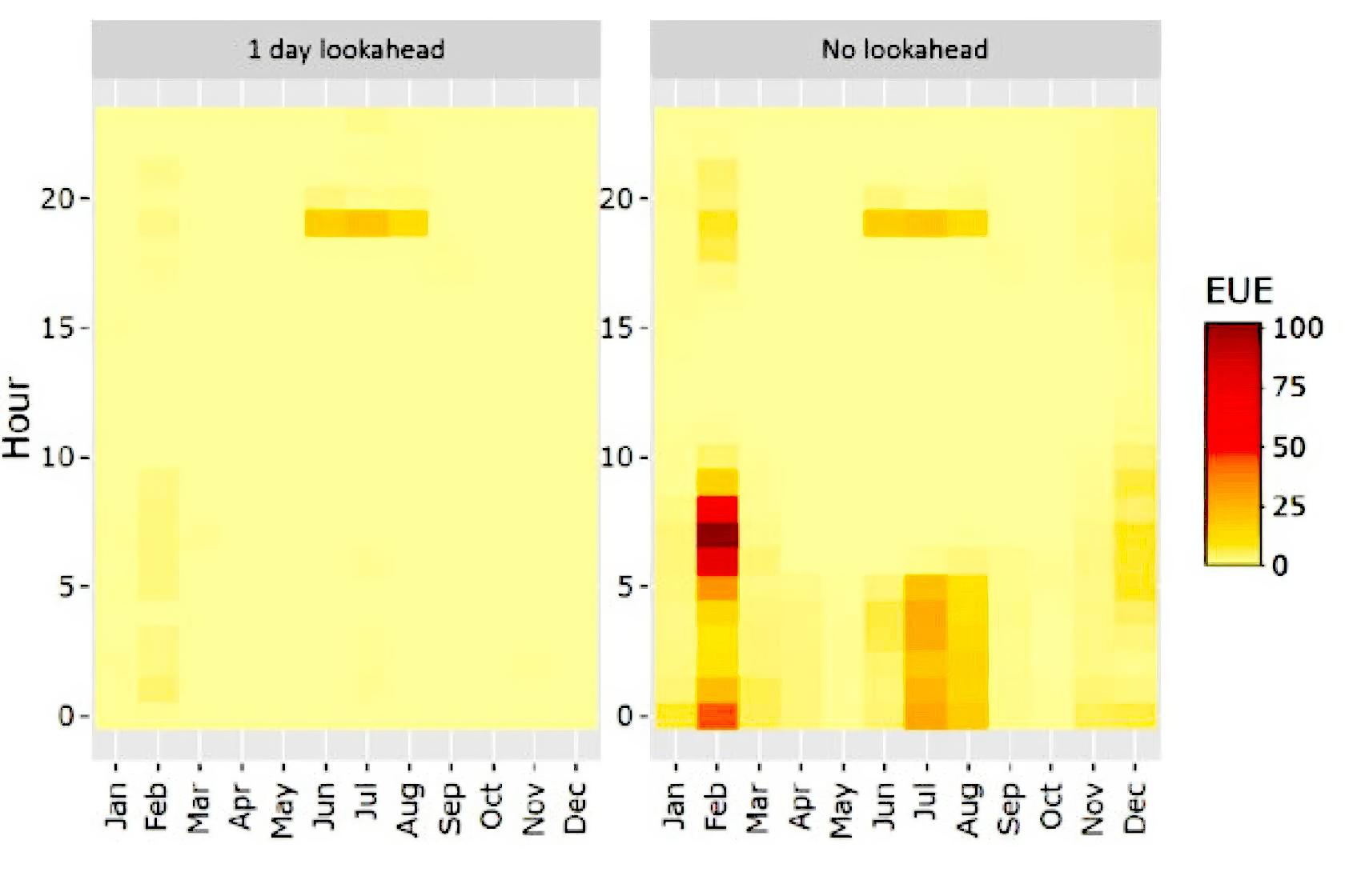
Figure: Month by hour of day EUE heatmaps for simulations with, and without, lookahead for a high VRE + storage portfolio
A Western US Case Study, also conducted as part of the Resource Adequacy for a Decarbonized Future Initiative, shows similar findings. Results are presented in the figure below. Five different total optimization windows (results + lookahead) were tested; the 1-day window has no lookahead, the 4-day window has a 3-day lookahead, and so on. These analyses were conducted on a high VRE system with a combination of 8-hour and long-term (multi-day) storage. Longer optimization windows reduce LOLE by better optimizing storage usage and preparing for highest system risk situations. However, care must be taken with over-optimizing storage operations, leading to overly optimistic results given that real-life foresight is limited. As such, shorter lookaheads, typically one week, were chosen for most of the analysis in that study, reflecting a case where week ahead forecasting is relatively accurate in terms of knowing overall energy needs on a day, but beyond that assumed less accurate.
Figure: LOLE as a function of lookahead for high VRE + storage portfolio
HYDROELECTRIC POWER
Background
Hydroelectric power is one of the oldest sources of electricity generation, with its introduction quickly following the invention of the electric generator. Worldwide installed hydro power capacity reached 1,360 GW in 2021, including 165 GW of pumped storage.1 Hydro power has several highly valuable characteristics for operations and resource adequacy:
-
It can be dispatchable.
-
It can provide long- and short-term energy storage.
-
Installations generally have high capacity and long lifetimes.
-
It is renewable and largely carbon free.
Hydro power plays a key role in RA in many parts of the world, with some systems being particularly dependent on it.
Hydro power dispatch is constrained by operational and environmental and regulatory constraints. A common set of these constraints are summarized in the table below.
|
Category |
Type |
Constraint |
Run of River |
Reservoir |
Closed loop PSH |
Open loop PSH |
|
Operational |
Turbine |
Max/min power (MW) |
X |
X |
X |
X |
|
Ramping ability (MW/min) |
X |
X |
X |
X |
||
|
Up/downtime (h) |
X |
X |
X |
X |
||
|
Reservoir |
Absolute capacity (MWh) |
X* |
X |
X |
X |
|
|
Quantity stored (MWh) |
X* |
X |
X |
X |
||
|
Pump |
Max/min power (MW) |
X |
X |
|||
|
Ramping ability (MW/min) |
X |
X |
||||
|
Up/downtime (h) |
X |
X |
||||
|
Environmental and Regulatory |
Flow |
Max/min flow constraint (m3/s) |
X |
X |
X |
X |
|
River flow variation (m3/s2) |
X |
X |
X |
|||
|
Reservoir |
Level restrictions (l or m3) |
X |
X |
X |
||
|
Restriction of prolonged storage (h) |
X* |
X |
X |
X |
||
|
* Applicable to RoR units with pondage |
||||||
Operational constraints capture the physical and technical limitations of hydro power plants. All forms of hydropower generation utilize turbines to generate electricity and are therefore limited by their technical specifications, including maximum and minimum power outputs, ramping capabilities, and turbine up and down times. Constraints relating to reservoir capacity apply to PSH, reservoir hydro, and RoR with pondage. Pump constraints only apply to pumped storage hydro, and include power, ramping, and up and down time constraints. PSH pump and turbine constraints can either be the same, or different, depending on specific unit characteristics.
Environmental and regulatory constraints arise from the opportunity cost of using waterflow, rivers and reservoirs for power generation versus using them for recreation, irrigation, human consumption, or as a habitat for wildlife. To balance needs across each of these uses, environmental and regulatory constraints are often imposed on hydro generation. To comply with environmental, regulatory, and operational restrictions on flow and flow variations, RA models may constrain power output or power output variation hourly, daily, or weekly.
Finally, climate change may not be explicitly considered today when modeling hydro generation, however it continues to impact hydro generator outputs. Impacts such as reduced icy seasons, greater precipitation during flood seasons, or reduced overall precipitation are affecting operator decisions, as well as altering patterns of water availability. As hydrologic conditions continue to change, models will need to reflect new restrictions on usage.
Any constraint may be implemented either as a hard or a soft constraint in RA and operational models, depending on its nature and the real-world repercussions of breaking it. Hard constraints cannot be broken by the solver and are used to represent physical limitations to hydro power operations, i.e., those related to physical reservoir size and storage capacity or turbine capabilities limitations on power outputs. Soft constraints may be broken, often at a high penalty cost. For example, excess water spillage may be allowed during a flood, at a penalty cost representing the cost of the fines that would be imposed in real life. The value of the penalty cost associated with each constraint determines the order in which constraints will be broken if needed to support system operations, with lower penalty costs broken first.
Models treating hydropower as a dispatchable resource and assuming a low variable cost value in their economic optimization run into problems appropriately dispatching reservoir hydro power. Hydroelectric generators have very low variable costs, especially when compared to thermal units. While entering RoR units into economic optimization models with zero cost ensures that their must-run generation is always taken, modeling close-to-zero cost reservoir hydro units would result in the immediate dispatch of hydro generation as soon as water is available. This would result in suboptimal hydroelectric resource usage, leading to periods requiring more expensive generators to be utilized and overall resulting in a suboptimal use of system-wide resources.
To allow for the optimization of hydro power over optimization windows as short as days or weeks, while considering the seasonal patterns of water inflow and electricity demand, historical data may be used directly to set water usage constraints. These constraints may also be calculated using heuristics or through preprocessing simulations. Pre-processing runs often involve running optimizations with timesteps greater than 1 hour, e.g., 4 hours, and use historical inflow, outflow, and reservoir level data to set appropriate usage constraints. These constraints are often implemented through:
- Energy allotments
- Reservoir trajectories
- Water values
Energy allotments limit hydro power generation by providing a discrete amount of energy that can be dispatched each week. Often, the hydro resources are constrained to dispatch exactly the allotted amount, with no, or minimal, carryover allowed between optimization horizons (see figure below), however some models do include iterations, in which the energy allotments can be adjusted and fed back into the dispatch model if shortfalls are found to occur.
Figure: Example of weekly allotted energy for a sample reservoir unit.
Reservoir trajectories are an alternative to the energy allotment method. Here, a target reservoir energy value, sometimes within an envelope of possible values, is provided. Targets, or values within the reservoir trajectory envelope, must be met at the end of each time period, for example each week (see figure below). Contributions to RA may be greater when allowing trajectory flexibility within an envelope, rather than constraining reservoir levels to meet discrete values.
Example: ERAA reservoir trajectory compilation
The 2021 European Resource Adequacy Assessment employs a pre-processing hydro optimization that provides weekly reservoir trajectory data to be used as input for the dispatch optimization, setting minimum and maximum reservoir levels for each week, which are then input into the RA model as soft constraints. If appropriate data is not available, TSOs may provide fixed weekly targets which are then used as hard constraints to ensure reservoir levels reflect real world behavior. Deterministic targets are the less preferred option as they restrict the ability of hydro power to provide real-time flexibility in the simulation.
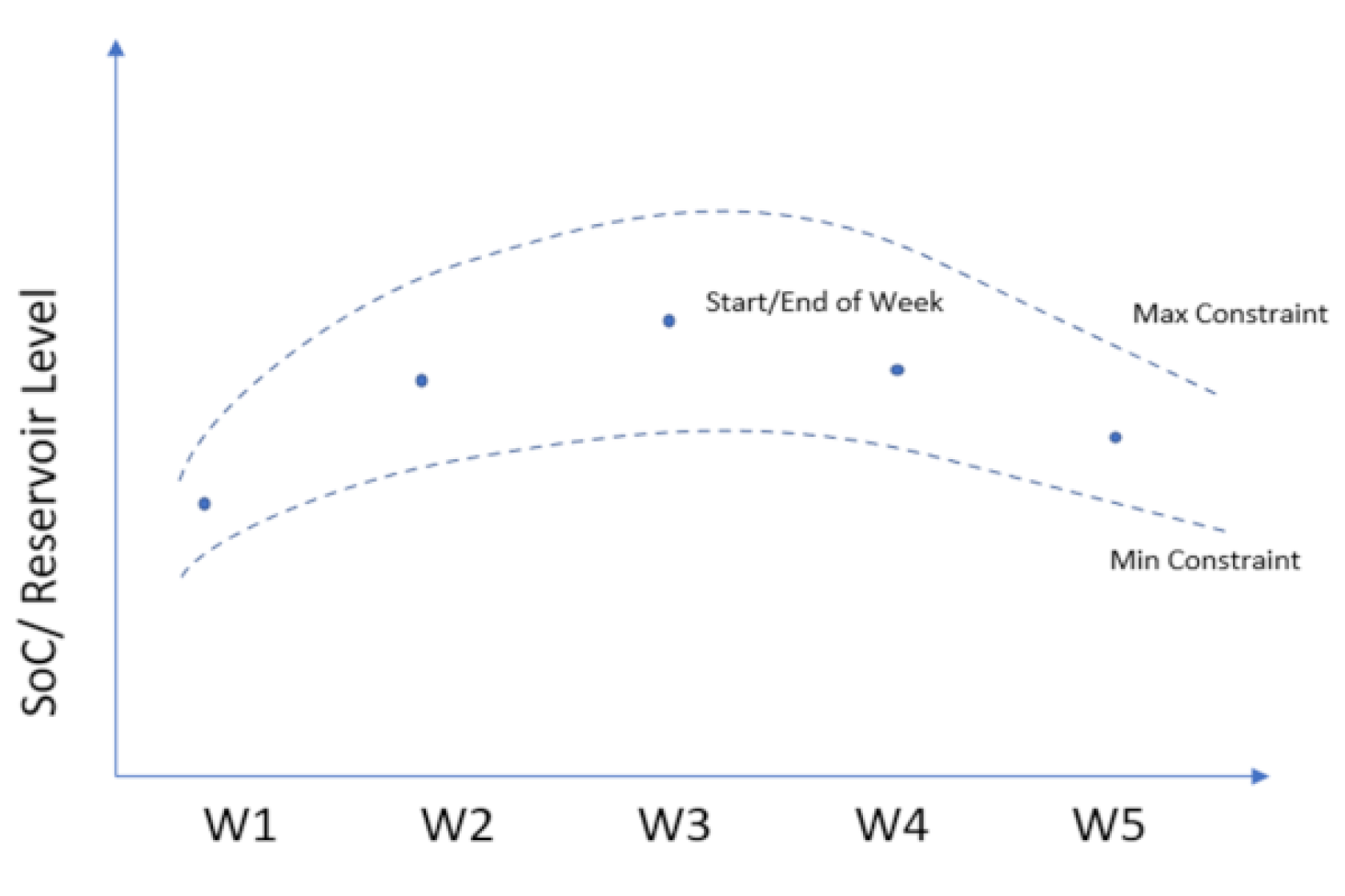
Figure: Month by hour of day EUE heatmaps for simulations with, and without, lookahead for a high VRE + storage portfolio
Water values are another tool employed by modelers to ensure that the opportunity cost of reservoir water usage is captured within RA. One option is to set fixed, seasonal, or monthly water values, and employ hard constraints on maximum and minimum generation. This method sets a value for reservoir hydro usage within the merit order. However, if system prices are sufficiently high, the reservoir hydro can still be inefficiently dispatched.
Another option is to use water value curves. Here, hydro reservoir water is discretized into several blocks, each of which have a different water value, as illustrated below. Water closer to the top of the reservoir will have low value to prioritize evacuation to make room for inflows. Water closer to the minimum reservoir level will be extremely highly priced, either high enough that it will never be dispatched, or alternatively, with a water value that will only be reached during severe contingency events, allowing it to provide emergency dispatch.

Figure: Month by hour of day EUE heatmaps for simulations with, and without, lookahead for a high VRE + storage portfolio
Water value curves can be obtained in three main ways: through user input based on historical data, via a preprocessing simulation, or by dynamically assessing the current reservoir status and hydro forecast during each optimization horizon. While user input and preprocessed curves require less computing power, dynamically generated curves can respond much better to system events, and more closely represent real world hydro operations.
It should be noted that there is a lack of consensus regarding best practices in reservoir management modeling. Nonetheless, drastic differences in the adequacy contribution of reservoirs can exist when employing different modeling approaches.
Read more:
1 "2022 Hydropower Status Report," International Hydropower Association, London, 2022.
Hydro power dispatch is constrained by operational and environmental and regulatory constraints. A common set of these constraints are summarized in the table below.
|
Category |
Type |
Constraint |
Run of River |
Reservoir |
Closed loop PSH |
Open loop PSH |
|
Operational |
Turbine |
Max/min power (MW) |
X |
X |
X |
X |
|
Ramping ability (MW/min) |
X |
X |
X |
X |
||
|
Up/downtime (h) |
X |
X |
X |
X |
||
|
Reservoir |
Absolute capacity (MWh) |
X* |
X |
X |
X |
|
|
Quantity stored (MWh) |
X* |
X |
X |
X |
||
|
Pump |
Max/min power (MW) |
X |
X |
|||
|
Ramping ability (MW/min) |
X |
X |
||||
|
Up/downtime (h) |
X |
X |
||||
|
Environmental and Regulatory |
Flow |
Max/min flow constraint (m3/s) |
X |
X |
X |
X |
|
River flow variation (m3/s2) |
X |
X |
X |
|||
|
Reservoir |
Level restrictions (l or m3) |
X |
X |
X |
||
|
Restriction of prolonged storage (h) |
X* |
X |
X |
X |
||
|
* Applicable to RoR units with pondage |
||||||
Operational constraints capture the physical and technical limitations of hydro power plants. All forms of hydropower generation utilize turbines to generate electricity and are therefore limited by their technical specifications, including maximum and minimum power outputs, ramping capabilities, and turbine up and down times. Constraints relating to reservoir capacity apply to PSH, reservoir hydro, and RoR with pondage. Pump constraints only apply to pumped storage hydro, and include power, ramping, and up and down time constraints. PSH pump and turbine constraints can either be the same, or different, depending on specific unit characteristics.
Environmental and regulatory constraints arise from the opportunity cost of using waterflow, rivers and reservoirs for power generation versus using them for recreation, irrigation, human consumption, or as a habitat for wildlife. To balance needs across each of these uses, environmental and regulatory constraints are often imposed on hydro generation. To comply with environmental, regulatory, and operational restrictions on flow and flow variations, RA models may constrain power output or power output variation hourly, daily, or weekly.
Finally, climate change may not be explicitly considered today when modeling hydro generation, however it continues to impact hydro generator outputs. Impacts such as reduced icy seasons, greater precipitation during flood seasons, or reduced overall precipitation are affecting operator decisions, as well as altering patterns of water availability. As hydrologic conditions continue to change, models will need to reflect new restrictions on usage.
Any constraint may be implemented either as a hard or a soft constraint in RA and operational models, depending on its nature and the real-world repercussions of breaking it. Hard constraints cannot be broken by the solver and are used to represent physical limitations to hydro power operations, i.e., those related to physical reservoir size and storage capacity or turbine capabilities limitations on power outputs. Soft constraints may be broken, often at a high penalty cost. For example, excess water spillage may be allowed during a flood, at a penalty cost representing the cost of the fines that would be imposed in real life. The value of the penalty cost associated with each constraint determines the order in which constraints will be broken if needed to support system operations, with lower penalty costs broken first.
Modeling Options
A commonly used simplification to represent hydro power in RA is unit aggregation. Hydro power generation is often aggregated at the watershed level. However, it may also be clustered by unit type, where PSH may be clustered with other, non-hydro storage resources. Potential issues associated with aggregation include the violation of constraints for individual units, incorrect evaluation of hydro capabilities and contributions to RA, and reduced ability to account for maintenance and outages. Certain models may carry out a post-processing step to check whether optimized hydro dispatches violate individual unit constraints, iterating through the problem as necessary until an acceptable solution, with no constraint violation, is found.1
Read more:
LEVEL I:
Hydro power units are aggregated by unit type or watershed connection. Constraints for individual units are aggregated and simplified.
LEVEL II:
Hydro power units are aggregated by unit type or watershed connection. PSH is represented individually. Simulation outputs are post-processed and new constraints are iterated back into the optimization if necessary to ensure that individual unit constraints are not violated.
LEVEL III:
Each hydro plant is modeled individually. A full set of applicable operational, environmental, and regulatory constraints are modeled for all hydro power units.
One of the key factors making hydro power modeling a complex area for planners and operators is that water flows can connect almost any combination of the three main plant types. When hydroelectric plants are connected, waterflows through one plant affects operations for all connected downstream plants. These connected hydro plant configurations are known as cascading hydro power.
To represent cascading hydropower in an RA model, the relationship between different units must be known. Water inputs to a given plant may be separated into inflows that are dependent on the operations of up-stream plants, and those that are not. Representing cascading behavior increases the accuracy of RA and operational models, however, many systems do not consider it as it can significantly increase modeling complexity and reduce computational tractability. The tradeoff between RA model tractability and hydro power representation accuracy needs to be considered on a system-by-system basis, based on the amount of hydro in the resource mix as well as the complexity of the hydro plant operations.
LEVEL I:
Cascading impacts on hydro operations are not recognized
LEVEL II:
Key cascading dependencies are recognized in the model. These need to be identified on a system-by-system basis.
LEVEL III:
Cascading impacts on hydro dispatch are recognized, including the distinction between cascading and non-cascading water inputs.
Nonetheless, it should be noted that detailed modeling of cascading hydro operations can be highly data and computationally intensive. This is only recommended for those systems that are heavily reliant on hydro, or where cascading hydro power plays a key role in RA.
Run-of-river (RoR) units generate electricity by diverting a portion of river flow through hydroelectric turbines. RoR generation is largely dependent on natural water flows as most plants do not have reservoirs. However, certain larger installations may have a small reservoir, known as pondage.
RoR shares certain key characteristics with VRE; generation is most often non-dispatchable (except for RoR with pondage) and dependent on hour-to-hour water inflow availability. RoR water inflow timeseries are often obtained from historical generation data. Other than water availability, RoR outputs are also constrained by operational, environmental, and regulatory considerations, as outlined in the table above.
Pondage RoR is rarely explicitly modeled in RA: pondage generation outputs are often considered through RoR water outflow timeseries. However, in systems with large pondage capacity, it may be necessary to model it explicitly as a form of reservoir to appropriately capture its capacity to provide system flexibility and RA support.1
Read more:
1 G. Iotti, "Hydropower Modelling in Mid-Term Adequacy Forecasts," Politecnico Di Milano, Milan, 2020.
LEVEL I:
RoR outputs are modeled through timeseries based on historical data, without explicit consideration for pondage
LEVEL II:
RoR outputs are modeled through timeseries based on historical data with expected pondage outputs integrated into timeseries.
LEVEL III:
Pondage is explicitly modeled as a reservoir connected to RoR operations. Pondage outputs may be dynamically modeled as part of an optimization or input through a lower resolution pre-processing run.
Pumped storage hydro (PSH) plants connect two water reservoirs, storing, and generating electricity by moving water from a low elevation to a high elevation reservoir, and vice-versa. Closed-loop PSH installations are not connected to an outside body of water, whereas open-loop PSH is connected to a natural body of water. As for other energy storage units, explicitly modeling linked dispatch and state of charge within 8760 optimizations is the best approach to capture PSH operations. Additional constraints, outlined in the table above, are added as needed. Although alternative modeling methodologies exist, these are often less accurate.
Additional considerations regarding the modeling of energy storage units are outlined in the Storage and Hybrid Power Plants section.
LEVEL I:
Virtual node model without consideration of state of charge, or dispatched employing heuristics.
LEVEL II:
PSH dispatch and state of charge are explicitly represented within 8760 optimizations.
LEVEL III:
PSH dispatch and state of charge are explicitly represented within 8760 optimizations, recognizing distinctions between closed and open-loop PSH.
Reservoir hydro power plants use a dam to store water in a reservoir for later use. Operators can choose when to generate electricity by opening the dam and running water through a turbine, subject to the operational, environmental, and regulatory constraints outlined in the table above. Energy availability is influenced by water inflows, as is for RoR, but also by reservoir capacity. Reservoir hydro power is dispatchable, and water used to generate energy may or may not equal water inflows.
LEVEL I:
Hydro reservoir outputs may be modeled through timeseries, implicitly accounting for output constraints and long-term energy management. Long-term reservoir management constraints are determined from historical data.
LEVEL II:
Hydro reservoir is dispatched as part of the optimization. Long-term energy management is achieved through the implementation of energy, reservoir or time based (e.g., seasonal, or monthly) targets. Long-term reservoir management constraints are determined from optimization or heuristic dispatch preprocessing.
LEVEL III:
Hydro reservoir is dispatched as part of the optimization. Long-term energy management is achieved through the implementation of:
- Energy allotments,
- Reservoir trajectories,
- Water value curves.
Long-term reservoir management constraints are determined from optimization or heuristic dispatch preprocessing. Water value curves are dynamically calculated as part of the optimization.
As with other forms of generation, outages can either be planned or unplanned/forced. Planned outages include periodic maintenance, scheduled upgrades, or minor repairs. Forced outages can include equipment failures, or shutdowns due to extreme weather conditions. The reader is encouraged to refer to the Thermal Generation section for a detailed description of planned and unplanned outages.
Outages can be represented in several ways. Maintenance and forced outages are generally considered separately. Maintenance outages may be deterministically input into the model when the timing of these is known, or pre-processing runs may be conducted to probabilistically schedule maintenance outages, based on a pre-established maintenance rate. Commonly employed methodologies to capture forced storage outages in RA involve:
- Considering a fixed Equivalent Forced Outage Rates on Demand (EFORd).
- Advanced methods consider probabilistic modeling of forced outages, through mean time to fail, and mean time to repair Mean time to fail and repair values may be adjusted depending on the type of unit, for example, longer mean times to repair may be considered for hybrid plants.
Several RA models do not explicitly account for hydroelectric outages, and instead rely on these being implicitly represented in input data through capacity derates.
Finally, it should be noted that while correlated outages are not often captured in RA, hydro generators may be particularly susceptible to these, particularly under cascading configurations, where outages affecting one unit may have an impact on downstream units which utilize the same water flows.
LEVEL I:
Generator outages are not explicitly modeled but are implicitly accounted for through input timeseries data.
LEVEL II:
Periodic planned outages are accounted for. Unplanned outages are accounted for through fixed EFORd rates. The impact of sedimentation on generator availability may be considered through capacity derates.
LEVEL III:
Periodic planned outages are accounted for. Unplanned outages are modeled using both mean-time-to fail and mean-time-to-repair rates. The impact of sedimentation on generator availability may be considered through capacity derates. Outages due to water shortages may be accounted for probabilistically, as well as correlated outages.
FIRM AND FLEXIBLE DEMAND
Background

From an operational and modeling perspective, demand, or total system load, can be divided into two distinct categories (illustrated above):
-
Firm or essential loads that have no, or very little price elasticity and are not responsive to market or dispatch signals. These loads may include:
-
Loads from all customers that are not exposed to incentives to modify their consumption in any way.
-
Commercial or industrial loads where any modification in consumption, or process interruption, can incur high costs.
-
Critical or uninterruptible loads.
-
Certain firm loads may have the technical capability to provide a certain level of demand-side flexibility but may remain firm due to a lack of exposure to demand response signals, as is the case for customers on flat rate tariffs.
-
Loads that are responsive to market and dispatch signals are classified into two sub-categories:
-
Flexible loads, comprising all load types that can increase or decrease consumption in response to price, or dispatch, signals. These loads do not need to make up for deviations from baseline consumption. An example may be dimming the lights at a commercial establishment in response to a price signal (i.e., time-of-use prices). Flexible loads can be permanently lowered after activation (i.e., the lights stay dimmed until the next day) or reset to their previous consumption levels. This category includes curtailable, as well as turn-up (load-building) loads, although the latter has been less commonly deployed to this date.
-
Shiftable loads, unlike flexible loads, need to make up for deviations from baseline consumption when providing demand flexibility. For example, electric vehicle charging may be deferred; however, vehicles need to make up for missed charging after a scarcity event is over. Shiftable loads may be compounding or non-compounding:
-
Non-compounding shiftable loads are typified by (smart) washing machine loads. The load is shifted from one period to the next, with no change in overall energy used.
-
Energy consumption of compounding shiftable loads changes based on the duration of the advance or deferral of consumption, relative to immediate use. Electric vehicles, energy storage, and electric heating and cooling can behave in this way, owing to efficiency losses or changing background variables such as weather. It should be noted that some non-compounding loads may become compounding if consumption has been deferred for a sufficiently long time.
-
Responsive Load Activation and Availability
Demand-side flexibility (DSF), or responsive demand, are both taken to refer to the capacity for responsive loads to respond to incentivized consumption changes, measured at the customer meter. There are two ways of activating DSF:1
-
Price-based programs use price signals or tariffs to incentivize consumers to flex or shift consumption. Prices serve as an incentive; the customer decides whether and when to respond. Price-based programs include time-of-use tariffs, critical peak pricing, demand charge programs and real-time pricing programs.
-
Dispatchable load programs where customers subscribe to programs allowing for certain loads to be flexed or shifted subject to a set of constraints limiting the timing, duration, or total energy that is dispatched. Dispatchable load programs include reliability dispatch, emergency load reduction, and interruptible load programs.
The way DSF is activated has implications on dispatch and therefore on modeling flexible loads in RA. The table below shows an overview of some of the key factors influencing responsive load behavior and availability, affecting operations and adequacy.
Table: Factors influencing responsive load behavior and availability.
Factors influencing response and availability |
Tariff or flexible dispatch incentive design Dispatch number and duration limits Weather Time of day Time of week Season Customer fatigue End-use technology availability Ability to flex or shift consumption economically and technically |
Read more:
Other related reading:
Modeling Options
The industry standard is modeling firm loads through forecast timeseries data. From a resource adequacy modeling perspective, the differences between Level I and Level III implementations are based on how uncertainty is considered. That is, whether, and how, multiple future load forecasts are accounted for.
Assuring the quality of firm load forecast timeseries heavily depends on the capabilities of load forecasting and scenario generation approaches.
Load forecasting involves the generation of (often probabilistic) future firm load timeseries based on predicted weather patterns (including impacts from anthropogenic climate change), economic factors, end-use technology and DER adoption, demographic change, the rollout of energy efficiency schemes, and other socio-economic factors potentially impacting electricity demand – not all these factors are used in current forecasts, but this is the general industry trend. Advanced load forecasting approaches may consider a wider range of weather years as well as track large industrial load, hydrogen generation, transport electrification and DER growth closely. Additionally, higher fidelity load forecasting accounts for weather-correlation across all weather-dependent timeseries, including wind and solar outputs, as well as generator outages.
Scenario generation tools then assure that the appropriate set of future load forecasts are selected and included in RA assessments such that a suitable range of risk is captured in models.
LEVEL I:
A fully deterministic model with limited firm demand uncertainty is used for modeling of firm loads.
LEVEL II:
A hybrid model considering multiple deterministic firm load uncertainty scenarios is used for modeling of firm loads.
LEVEL III:
A probabilistic model considering a range of possible future load scenarios and weather-correlation across all weather-dependent timeseries is used for modeling of firm loads.
The most employed method for capturing responsive load impacts on resource adequacy is through the inclusion of static timeseries, aggregating expected demand-side response across a range of demand-side programs. This approach assumes that customer behavior is consistent in response to consistent signals, which are not always influenced by real-time system conditions. Response is modeled in a static manner, meaning that it is pre-determined and exogenous to internal RA optimizations.
Static modeling is appropriate for capturing demand-side flexibility that is responsive to signals that are consistent over time and that do not necessarily reflect real-time system conditions. For example, customer response to time-of-use tariffs is best captured using static approaches. However, this approach underestimates the potential capabilities of DSF able to provide flexibility in response to real time or near real time signals – this can become important for RA given these may reflect scarcity conditions. The lower complexity and computational burden of aggregated static modeling may be acceptable under low DSF rollout scenarios but will likely misrepresent flexible load operations under higher rollouts.
Dynamic models represent responsive demand endogenously in RA, capturing the ability for loads to respond to real-time system conditions. The flexible generator modeling approach is often used, representing responsive loads through a pseudo-generator with unlimited ramping capability and dispatching at a set activation price. Today, the flexible generator model is mostly used to represent emergency demand response programs, such as critical peak pricing and emergency load reduction programs. The activation price for responsive demand is often higher than that of most other generators, ensuring that demand-side flexibility resources are exclusively used as a contingency resource. However, dynamic modeling is also appropriate to represent day-to-day responsive load operations from loads subscribing to programs such as real-time pricing.
An additional consideration is that dynamic models today mainly model flexible loads but do not model shiftable response (see figure below). However, responsive shiftable loads are likely to rapidly grow; electric vehicles, heat pumps, and electric water heaters all require load shifting when operated flexibly. That is; any deviation from their baseline consumption needs to be made up for. Load shifting can have impacts on RA that need to be carefully studied given that moving consumption from one period to another could also shift RA stress periods.
Finally, there is an inherent uncertainty in responsive load behavior, particularly under programs when customers decide when and how to respond to signals. Advanced representations, both static and dynamic, recognize this uncertainty and deploy probabilistic models based on historical response data.
Highest fidelity models match demand-side response programs to their appropriate, static, or dynamic probabilistic representations.
LEVEL I:
A static timeseries approach applied to model aggregated response from all responsive loads.
LEVEL II:
Most responsive loads for are modeled using a static approach, however dynamic approach may be used to represent emergency load curtailment programs.
LEVEL III:
Both static and dynamic approaches are used and are matched to the appropriate demand-side response programs. Load building programs are considered as well as load reduction. The probabilistic nature of demand-side response is modeled.
When static timeseries modeling approaches are selected to represent responsive loads, operational constraints are assumed to be implicitly captured in the input timeseries and are not explicitly modeled as part of RA optimizations. While simpler to model, this will miss some of the key characteristics of demand flexibility that can support adequacy, particularly when it comes to representing loads that respond to real-time, or close to real-time signals. However, when responsive loads are modeled dynamically, an explicit formulation of operational constraints is required in order to accurately capture demand-side response contributions to adequacy. Accurately capturing DSF constraints can be especially relevant when modeling programs that target response from a particular technology, such as smart thermostat reliability dispatch programs. A summary of modeling considerations and constraints, specific to static and dynamic models can be found in the figure below.
Constraints applied to dynamic responsive load models can be divided into those that apply to both flexible and shiftable loads, and those that apply exclusively to shiftable loads, as illustrated below.
LEVEL I:
Flexible load response is modeled statically, and availability constraints are assumed to be implicitly captured in timeseries.
LEVEL II:
Certain constraints are applied to dynamically modeled flexible loads.
LEVEL III:
All relevant constraints are applied to dynamically modeled flexible and shiftable loads.
Figure: Modeling considerations, constraints, and parameters for static and dynamic responsive load models.
Open Modelling Gaps
Since the explicit inclusion of flexible loads in resource adequacy assessments is nascent, gaps in data collection and establishing modeling approaches remain.
For example, modeling response degradation, due to customer fatigue, or other, as well as weather-dependent demand-side response is incipient and industry standards have not been established yet. Data based on trials or real-life programs quantifying the impact of customer fatigue, technology-based factors, or extreme events on demand-side response is hard to come by, and therefore models accounting for response degradation or weather-dependent demand-side response are rare. However, understanding how customer response may degrade and the factors influencing degradation, as well as weather impacts on response will be imperative in the future, particularly if systems are to rely on responsive loads for operations and adequacy.
DISTRIBUTED GENERATION AND STORAGE
Background
Distributed generation and storage encompass any small, generally less than 10 MW, generation and storage resources located behind the customer meter. Only those technologies who’s end-use is to generate or store energy are addressed in this section, focusing on distributed PV, distributed energy storage, and co-generation, also known as combined heat and power (CHP).
The key additional challenge arising when modeling certain distributed assets is that system operators may have limited visibility of installations and their operation. Data collection challenges related to distributed resource modeling are addressed in the Data Collection page.
Modeling Options
At low distributed PV shares, heuristic approaches, netting expected distributed PV generation from demand based on averaged irradiance patterns may suffice. At higher shares, distributed PV requires similar treatment to bulk system installations, including the generation of forecasts based on several years to decades of hourly historical PV output data. Additionally, care should be taken to ensure correlated weather year data is used across all weather-dependent technology and load models.
An additional consideration when modeling distributed PV is that while optimal pitch angles are obtained with large-scale solar installations, they are not always possible with rooftop PV, leading to lower power outputs. The influence of distributed PV pitch angle on generation, and other factors such as shading from trees or overhead lines, as well as lower maintenance levels resulting in increased outages, may need to be explicitly considered when forecasting distributed PV outputs at high rollout levels.
LEVEL I:
Heuristic approach netting distributed PV generation from demand based on expected irradiance.
LEVEL II:
Distributed PV outputs are modeled based on several years of historical hourly PV output timeseries data.
LEVEL III:
Distributed PV output forecasts are generated based on several decades of hourly data, with correlation amongst weather shapes enforced. The impact of pitch angles on PV outputs is accounted for.
Customer-located distributed storage is most found connected to PV systems. Many adequacy assessments account for distributed PV, however, those explicitly modeling distributed storage are rare.
Many of the considerations for modeling short-term storage developed in the Storage and Hybrids section of this site apply to distributed storage, however, operational strategies can significantly differ between bulk and distributed storage. Customer-located storage is largely dispatched to minimize customer electricity costs, regardless of whether operations support the bulk system or not and is therefore heavily influenced by customer demand and solar power availability.
At very low levels of distributed storage shares, the impact of distributed ES on net demand may be considered using heuristics, assuming that most customer-located distributed storage assets reduce net consumption in the early morning and evening, at times when there is no PV output, or it is low. At higher levels of distributed ES rollouts, static storage profiles may be generated based on years of historical PV output data assuming that batteries are largely charged from excess rooftop solar and discharged when household load exceeds rooftop PV production, accounting for storage roundtrip efficiency losses. Alternatively, when historical distributed storage operation data is available, forecasts may be built based on existing data.
The highest fidelity modeling involves understanding how storage responds not only to customer demand and PV availability, but considers how customer tariffs, including adherence to time-of-use or net-energy metering may impact response.
LEVEL I:
Heuristic approach netting estimated storage outputs from load based on averaged demand and distributed PV profiles.
LEVEL II:
Storage static profiles are generated based on years of historical PV output data assuming that batteries are charged from excess rooftop solar and discharged when household load exceeds rooftop PV production. Battery roundtrip efficiency is accounted for.
LEVEL III:
Distributed storage static forecast timeseries are generated based on decades of historical data accounting for weather-correlated distributed PV outputs and battery roundtrip efficiency.
Customer net-energy metering tariffs may be considered when forecasting distributed storage operations.
Combined heat and power (CHP), or cogeneration, refers to the same technology. Both describe the simultaneous generation of electricity and heat serving (partially or completely) commercial, industrial, and district heating loads that would otherwise be largely served by the grid. CHP units are mainly gas-fueled, although dual-fuel plants also exist to enhance fuel security.
For systems with low CHP rollouts, accounting for its impacts on demand implicitly through net load profiles may suffice. At higher CHP rollout levels, some level of differentiation between flexible and inflexible CHP units may be necessary. Small, non-dispatchable units may be modeled as must-run units based on historical generation data. Larger, dispatchable CHP units should be considered separately. These units may be modeled using partial must-run constraints while allowing some flexibility to meet bulk-system needs.
Systems with high levels of CHP rollout may require similar modeling considerations to those outlined for thermal generation, including more detailed modeling of planned and forced outages, weather impacts on operations, as well as energy limits due to fuel availability.

CHP Power to Heat Ratios and Flexibility
CHP units can be more power- or heat-driven. Power to heat ratios are used to express the relationship between power and heat CHP outputs. Inflexible pure back-pressure CHP units have fixed power to heat ratios. Other CHP plant types, often larger CHP units such as extraction/condensing turbines, offer more flexible operations and can vary their power to heat ratio.
Many small-scale CHP units are designed as baseload and are operated to meet customer heat demand making them inflexible, must-run capacity. Baseload operations grant these CHP plants forced outage rates that are often lower than those of bulk system gas units.
LEVEL I:
CHP impacts on the net load are implicitly accounted for in net-load timeseries but are not explicitly modeled.
LEVEL II:
CHP units are explicitly modeled as part of RA.
Some differentiation between flexible and inflexible CHP plants may be considered.
LEVEL III:
CHP units are explicitly modeled in RA, separately capturing operations from inflexible and flexible plants.
Flexible operations are captured by enabling the ramp up of production and exporting power to the grid under power shortage situations or ramping down production under excess generation and low market prices.
CHP asset availability, weather impacts on operations, and energy limitations may be considered.
TRANSMISSION NETWORK
Background
Although onshore wind, offshore wind, solar PV, and concentrating solar power are all different technologies, they are modeled similarly within resource adequacy studies and therefore addressed together here. Because of the dependence of variable renewable energy (VRE) on stochastic weather phenomena, representing VRE generation is an important source of uncertainty to capture in RA modeling. Unlike technologies like coal, natural gas, and nuclear generation, the output of VRE is strictly dependent on environmental factors: mainly wind speed and solar irradiance. Historically, VRE outputs have been treated as non-dispatchable resources: they could be curtailed but did not generally participate in real-time electricity markets. However, with the development of advanced control strategies, VRE units can provide a range of grid services, including frequency regulation and synthetic inertia, much like conventional generators, within the envelope allowed by varying environmental conditions.
Modeling Options
In power system modeling tools, transmission network representations are generally split into three categories of complexity: nodal, zonal, and copper sheet. While nodal topologies provide the most accurate reflection of the actual power system, they are also the most complex to solve and require the most data. As for many of the other technologies considered in this report, there is an inverse relationship between model complexity and simulation runtime. Factors such as system size, model runtime/performance, and study intent factor into the decisions for which model type is used.
In 2016, MISO performed an exploratory nodal RA analysis which observed that loss of load events occurred at 11 buses of the 8,635 that were modeled, identifying local issues that would have been missed with a less granular transmission model.1 However, MISO staff also noted that the simulation required approximately 140 hours to evaluate 1000 samples for a single week, a substantial computational burden. Despite growing adoption of cloud computing, advancements to computational hardware, and software parallelization, such an exercise may still require a substantial amount of time to be performed. As such most resource adequacy models do not contain a nodal level of granularity.
Read more:
LEVEL I:
A copper sheet model is used.
Many planning studies utilize a copper sheet, or copper plate, model that does not represent any intraregional transmission infrastructure limits in resource adequacy. In this approach, all transmission constraints are unaccounted for by connecting all loads and generators to a single, lossless bus. While this type of simplification allows for the fastest runtimes, not accounting for transmission constraints may underestimate reliability risks. By definition, a true copper sheet analysis would only evaluate generation supply adequacy since no transmission data is considered.
A key issue that arises with copper sheet models is that, while system-level shortfall events are reported, information about where they are located is missed. If a zonal model is used instead, information about where system events occur is available, along with information on whether individual events occur due to insufficient generation or transmission limitations.
LEVEL II:
A zonal model is used.
In zonal models, systems are divided into regions separated by the major transmission corridors. The interface limits between the zones are often determined up-front using production cost models simulating the network in detail. Zonal models simplify the grid model by assuming point-to-point HVDC connections between zones, and copper plates within each zone. The model implemented often follows a ‘transport model’ approach, limiting flows based on import and export limits, but does not have regard for the physical flow of electricity across an AC system.
LEVEL III:
A flow based zonal or nodal model (if relevant) is used.
In an advance on the zonal approach, flow-based zonal models can be implemented where the inter-regional transfer limits are based on a reduced order model of the transmission system (AC and DC). In this type of model, regard is given to the physical flow of electricity by considering some version of a power flow: this could be DC power flow, linearized AC, or full AC power flow in limited cases.
A nodal transmission model contains data for each bus, transmission line, and transformer on the transmission network. Typically, nodal analyses are used together with DC power flow analyses and detailed production cost models in operational settings.
Transmission outages are another important consideration for overall system adequacy. If the transmission system is modeled as lossless, but large outages are observed in real-time impact regional transfer capabilities, then the model is likely under-estimating loss of load risk. Such outages could be caused by insulator failure, environmental events, or other equipment failures. For a nodal model, adding outage rates is straightforward, but this is complicated in zonal models since multiple lines may aggregate to the interface modeled between zones. Choosing if, or how, to incorporate transmission outages into the model may impact the nature of reliability risk. For example, NYISO uses a zonal model and assumes all overhead lines are always available but that underground transmission cables are subject to failure. In their model the individual cables are bundled and many derate levels are modeled with associated probabilities of likelihood.1
Read more:
1 New York ISO, "2022 Reliability Needs Assessment (RNA): Appendicies," Rensselaer, NY, 2022.
LEVEL I:
Network outages are not modeled, or not applicable since copper sheet models are used.
LEVELS II & III:
Network outages are modeled in zonal and nodal transmission network representations.
In studies utilizing a zonal model, each zone is typically connected to at least one other zone by a line that has representative transmission limit applied. These limits must be calculated in careful consideration of the existing transmission network and are a critical modeling component. However, depending on the system, some zones may be connected to multiple zones. While each individual interface has a limit, there may be a need to model a joint limit between two or more interfaces to reflect additional limits in the underlying transmission system. For example, consider two 100 MW lines entering a zone but a joint import limit of 160 MW. By excluding this joint limit, a resource adequacy event could be missed. Zonal models that do not account for joint import/export limits may underestimate reliability risk.
Further, transmission lines can have different limits in real time operations depending on ambient conditions, series compensating devices, or whether specific resources are providing voltage support. If a line limit in an RA study is set at its annual maximum value and does not consider factors that could reduce its limit, then events caused by transmission limitations can be missed. For example, NYISO has periodically evaluated the sensitivity of a group of lines that are subject to a voltage limit that can change depending on which units are online.1 A simplified version of this model is incorporated into their RA analyses to reflect the importance of unit availability on the transmission system. While the representation of the interface in the RA model is simplified, the value is based on separate, exogenous, and highly detailed AC power flow analysis. Failure to account for time-varying or other large impacts in transmission limits may result in underestimating reliability risk. Similarly, always using the most restrictive representation of a limit may overestimate reliability risk and lead to unnecessary mitigation at great cost to consumers.
Read more:
LEVEL I:
Network outages are not modeled, or not applicable since copper sheet models are used
LEVEL II:
Models fixed transmission line limits. May recognize joint import limits.
LEVEL III:
Models time-varying transmission line limits and joint import limits.
Case Study: Transmission Between and Within Regions in RA Assessment
EPRI examined the implications of transmission in two different case studies to examine different issues.
In the case study based on the Midcontinent US system, a transfer analysis was carried out to examine the benefits of transfer capability between North and South MISO. This first required a zonal model between the regions to be developed, starting with an arbitrarily large constraint (10,000 MW in below figure) at which there is a 0.1 LOLE, and then gradually lowering the capability to zero. As can be seen, somewhere around 7500 MW, separation between the zones occurs, with the North zone seeing a shortfall and south seeing an excess (though across the system, LOLE was larger as a whole as transmission capability reduces).
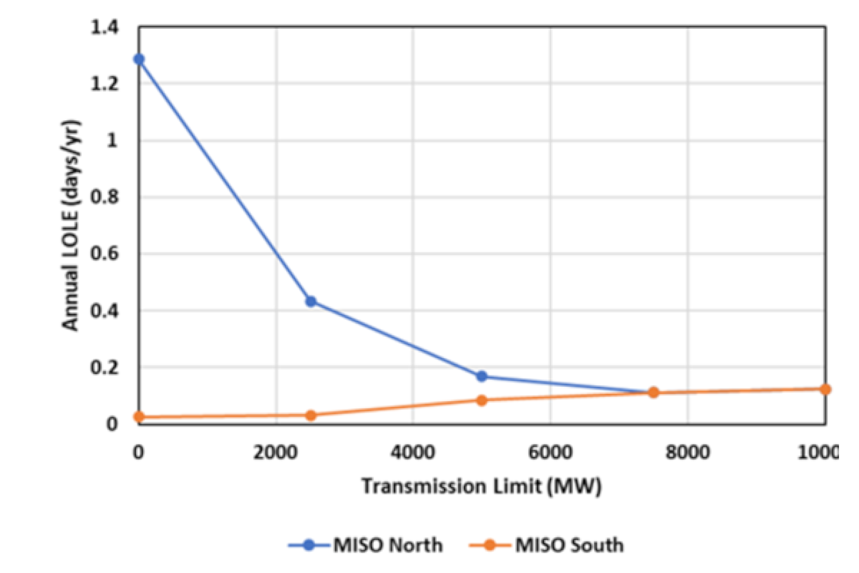
Figure: Impact of internal transmission in MISO region, between North and South.
This can be extended to the concept of an ELCC for transmission, where the benefits of transmission to both sides of the constraint can be recognized as the additional load that can be carried based on the transmission. More details are provided in the relevant report, but in summary it was shown that, as risk periods were not entirely coincident across both sides of the north-south constraint, the increased in transmission capability could result in an ELCC equivalent to more than the transfer capacity, i.e. an ELCC of greater than 100%, as it can provide support on both sides of the constraint, particularly when the limits are lower.
The examination of zonal levels of outages and LOLE also brought up the question of how unserved energy is allocated in models – whether equally shared with assumption of copper plate, based on load in the region, or based on the balance prior to transfers. In the case of equal shares, when transmission is included, it can result in non-convergence. However, that is often the default method used in studies. As such, it would be recommended to allocate outages based on the resource balance prior to transfer. This better allows for identification of where the shortages might be and can be addressed by either additional transmission or increased resources within the region (which should be studied for economics and capability to build transmission).
In the Northeast US and Canada case study, implications of changing intra-region and inter-regional transmission between the six balancing authorities modeled were also examined. There, each region was included in the overall model, with inter-regional and intra-regional constraints included. Each individual region was brought to criteria of 0.1 LOLE, allowing for neighbors to support through an iterative modeling process, where each region is modeled first, and then available energy transferred between regions.
Figure: LOLE as a function of lookahead for high VRE + storage portfolio

GAS NETWORKS
Background
With the growth in wind and solar power, many systems have increased their reliance on gas power plant flexibility to balance net load variations. Gas is one of the primary fossil fuel sources used for power generation today. Gas is usually delivered “just in time”, with a limited amount of plant on-site storage capabilities. As such, the gas and power sectors are highly intertwined in day-to-day operations.
Key Components of Gas Networks
- Production fields
- Liquid Natural Gas (LNG) terminals
- Underground gas storage facilities
- Pipelines
- Compressor stations (to compensate for pressure losses across pipelines)
- Cross-border entry and exit stations
- City gate stations (where gas enters the distribution chain)
- Stations of direct served customers
Modeling Options
The challenges for planning and operations associated to the increased dependency of the power sector on the gas sector have been flagged by regulatory bodies, including NERC.1 Despite this, most RA studies do not explicitly model gas networks today. This is often due to a combination of lack of reliable data, computational limitations, and lack of appropriate simulation capabilities.
However, appropriately representing gas networks in RA studies would allow for a deeper understanding, and pathways to mitigation for adequacy issues including those arising from:
- Gas deliverability issues arising due to weather-dependent outages of the gas infrastructure.
- Gas deliverability issues related to insufficient gas supply.
- Ramping flexibility constraints related to offtake pressure requirements and gas transport lags.
Read more:
LEVEL I:
At level I an implicit gas network model through gas plant capacity derates informed by historical data is used.
In most adequacy models, constraints in gas availability and deliverability are not considered, nor is the gas network represented. This is a similar approach to the copper plate transmission network assumption described in the transmission model section, whereby gas is assumed to always be available when needed. However, motivated by the increasing reliance on gas for power generation, some studies do implicitly account for potential gas network issues. This is mainly achieved at present by de-rating gas units, where capacity de-rates are calculated based on historical observations including past gas network outages, fuel inventory limits, and gas offtake pressure constraints limiting ramp rates.
Implicit modeling approaches partially capture gas network constraints without including a full representation of the gas network, lightening the computational burden of RA assessments, and limiting the scope of the data collection and modeling work. However, this methodology does not provide information on the root-cause of gas-related outages. That is, no distinction is provided between plant outages, network outages, fuel insufficiency, or pressure-related issues. As such, it limits the capability for planners to devise targeted siting and network hardening actions to improve system adequacy.
LEVEL II:
At level II a fuel pool model is used.
Fuel pool modeling is where fuel consumption is exogenously energy-constrained based on daily or weekly intervals. This method allows for explicit differentiation between energy-related (i.e., insufficient fuel) and capacity-related (i.e., gas plant maintenance outages) outages, while abstaining from developing mathematical models representing gas networks.
LEVEL III:
For level III steady-state or linearized transient gas network models are used.
The two predominant approaches for explicit gas network modeling are steady-state and transient flow (or dynamic) models.
Steady-state models rely on the assumption that the gas in pipelines is incompressible, i.e., the inflow to a pipeline equals the outflow at each timestep. Depending on how sophisticated a model is, only transport capacities may be limited (i.e., transport model), or other constraints, such as pressure constraints, may be accounted for. The main advantage of this approach is that it can be formulated as a linear, convex optimization problem that could be integrated into RA models, provided sufficient data availability. However, since steady-state models do not capture non-linear gas behaviors, such as gas compressibility, certain pressure-related constraints (i.e., insufficient gas offtake pressure) are missed in steady state models.
The most advanced method to simulate gas networks is through transient gas flow models, also known as hydraulic gas network models. Here, dynamic flow of gas is represented through a set of non-linear non-convex equations. This type of model is not only able to capture constraints related to gas network topology, but also line pack flexibility, that is, how much gas can be stored and withdrawn from the gas network, depending on pipeline pressure. Furthermore, transient gas flows are explicitly captured as a function of pipeline geometry and network pressure differentials. While the level of detail provided by these models is high, their non-linear non-convex nature is highly computationally intensive and cannot be directly solved within a resource adequacy model today. To account for gas network constraints identified through hydraulic models in an RA model, these can be iteratively run for selected stress time periods. It is also possible to linearize and convexify full hydraulic models, while mostly preserving line pack and dynamic flows, that could then potentially be directly integrated in RA models.2
Modeling Gaps
One of the most challenging gaps when it comes to incorporating gas networks into RA models is the lack of gas network data availability, which is further discussed in the Data Guidelines (Coming Soon) section of this site. Additionally, to the best of our knowledge, no industry guidelines have been set, containing thorough quantitative analyses comparing the value of the different gas network modeling approaches for different power system configurations, making it difficult to estimate which level of detail is required for different types of RA assessments. Finally, few tools exist providing the capability to link power system models with transient gas models, and those that are available may lack resource adequacy functionality.
Resource Adequacy Fuel Insufficiency Screening Tool (RAFIS)
EPRI has developed a screening tool that takes information about how much gas is available through firm and non-firm contracts, the temperature dependence of non-firm contracts and how much gas is available based on firm and non-firm power and gas storage. It then examines gas generation, dual fuel capabilities and the rest of the system (load and other generation), to provide a first pass estimate of how much gas availability constraints may impact on loss of load, including whether dual fuel is recognized. While not a full probabilistic RA assessment, this can allow for an initial understanding of the potential for gas limits to impact on adequacy, and how different solutions (gas pipeline, gas storage, dual fuel, and firm contracts) may potentially help reduce risk. It can also be used to develop inputs for implicit modeling in the more detailed RA assessments.
HYDROGEN
Background
While hydrogen generation through electrolysis has existed for many decades, the use of hydrogen in the power sector, as well as interest in the large-scale deployment of electrolyzers is nascent. As such, the higher fidelity modeling approaches outlined below are likely unjustified at current electrolytic H2 production shares in most systems but may become relevant in the coming years as electrolysis and hydrogen use for power applications becomes more widespread.
Existing Processes for Hydrogen Production
The two main processes used to produce hydrogen are steam methane reformation and electrolysis.
In steam methane reformation, methane (CH4) reacts with high-temperature steam, splitting into hydrogen and carbon dioxide.1 Carbon capture and storage may be considered to reduce the carbon footprint of this process, although this is not common practice today. Steam methane reformation requires heat input, often from on-site generation or heat exchangers connected to other processes.
The process of electrolysis uses electricity to split water molecules into hydrogen and oxygen, collecting oxygen at the cathode of the electrolyzer and hydrogen at the anode. The main biproduct of electrolysis is oxygen. Different types of electrolyzers exist for hydrogen production, each having different operational constraints. These include:
-
Alkaline
-
Polymer Electrolyte Membrane (PEM)
-
and Solid Oxide Electrolyzer Cell (SOEC)
Alkaline and PEM are both commercially mature technologies, whereas SOEC is not yet commercially ready.2
Both alkaline and PEM electrolyzers offer a certain level of operational flexibility, while SOEC is not currently able to do so. Alkaline electrolyzers are the most mature and cost-effective technology today, but it is expected that the costs and efficiencies of PEM will improve over the next decade, making them competitive with Alkaline electrolyzers.2 Even though both alkaline and PEM technologies can provide flexibility, PEM have faster ramp rates, and start-up and shutdown times, making them better candidates for operations in systems with high VRE shares and high net-load variability (see table below). However, SOEC technologies may provide higher efficiency processes than existing technologies and offer the possibility to operate in reverse mode (i.e., as a fuel-cell) as they mature.
Table: Current technology performance characteristics for alkaline and PEM electrolyzers
|
Alkaline |
PEM |
|
|
Load range |
10 – 110% of nominal load |
0 – 160% of nominal load |
|
Start-up (warm – cold) |
1 – 10 minutes |
1 second – 5 minutes |
|
Ramp up and ramp down |
0.2 – 20% per second |
100% per second |
|
Shutdown |
1 – 10 minutes |
1 second – 5 minutes |
Read more:
2 ENTSO-E, "Potential of P2H2 technologies to provide system services," ENTSO-e, Brussels, 2021
Modeling Options
Representing Electrolyzer Loads
When connected to the system, electrolyzer loads need to be considered, either implicitly in load shapes, or explicitly as part of the dispatch model.
LEVEL I:
Electrolyzer loads are implicitly accounted for in net-load timeseries. Electrolyzer demand is assumed to be firm.
LEVEL II:
A small number of key characteristics of electrolyzer loads (i.e., minimum, and maximum power outputs) are explicitly modeled in RA and their potential to provide demand-side flexibility is recognized. No detailed distinction between electrolyzer technologies is considered.
LEVEL III:
Detailed constraints including ramp rates, overloading capabilities, and partial load efficiencies are considered for each electrolyzer technology. If demand flexibility is provided, unit-specific dispatch prices are accounted for.
Hydrogen may be used directly for power generation by blending H2 into gas networks or combustion chambers in gas-fired units, or by using fuel cells. The availability of hydrogen fuel is directly linked to energy adequacy. If hydrogen production is tied to renewable energy outputs, hydrogen availability may be variable unless it is firmed with additional renewable energy buildouts or back-up storage units.
LEVEL I:
Projected hydrogen generation may be modeled statically using timeseries. Fuel availability constraints are not considered. No distinction between generator types is provided. Outages are not modeled.
LEVEL II:
Power generation using hydrogen is explicitly modeled within 8760 optimizations. Some level of fuel availability constraints may be recognized through fuel pool models.
LEVEL III:
Power generation using hydrogen is explicitly modeled within 8760 optimizations. Fuel availability constraints are recognized and implemented using hourly offtake limits or fuel pool models. Appropriate constraints and outage rates are modeled, making the distinction between fuel cells and gas-fired generation.
Hydrogen storage has been attracting interest for electricity balancing, particularly long-term storage. There are several different technologies for storing hydrogen that are currently under consideration to meet the expected increase in H2 demand over the coming decades. Common options include high pressure storage vessels, liquid hydrogen, chemical hydrides (such as ammonia and methanol), and metal hydrides. Hydrogen storage is subject to similar modeling considerations as existing long-term energy storage, including optimizing the usage of long-term fuel stocks, energy losses and fuel leakages in the hydrogen conversion process, potential storage unit degradation, and accounting for simulation optimization window and end-condition impacts.
LEVEL I:
Hydrogen storage is not considered. Fuel is assumed to be available when needed.
LEVEL II:
Long-term hydrogen storage is modeled, and reservoir management constraints are applied.
LEVEL III:
Long-term hydrogen storage is modeled, and reservoir management constraints are applied. Storage technology-specific considerations are accounted for, including operational constraints, storage leakage, and fuel conversion efficiency. Impact of optimization windows and end conditions are considered.